How to Make Bar Graph of Continuous Data R Count
Bivariate Graphs
Bivariate graphs display the relationship between two variables. The type of graph will depend on the measurement level of the variables (categorical or quantitative).
Categorical vs. Categorical
When plotting the relationship between two categorical variables, stacked, grouped, or segmented bar charts are typically used. A less common approach is the mosaic chart.
Stacked bar chart
Let's plot the relationship between automobile class and drive type (front-wheel, rear-wheel, or 4-wheel drive) for the automobiles in the Fuel economy dataset.
library(ggplot2) # stacked bar chart ggplot(mpg, aes(x = class, fill = drv)) + geom_bar(position = "stack") 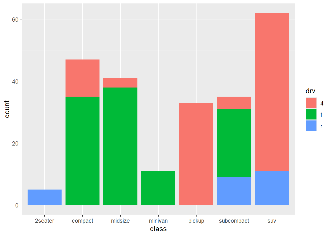
Figure 4.1: Stacked bar chart
From the chart, we can see for example, that the most common vehicle is the SUV. All 2seater cars are rear wheel drive, while most, but not all SUVs are 4-wheel drive.
Stacked is the default, so the last line could have also been written as geom_bar().
Grouped bar chart
Grouped bar charts place bars for the second categorical variable side-by-side. To create a grouped bar plot use the position = "dodge" option.
library(ggplot2) # grouped bar plot ggplot(mpg, aes(x = class, fill = drv)) + geom_bar(position = "dodge") 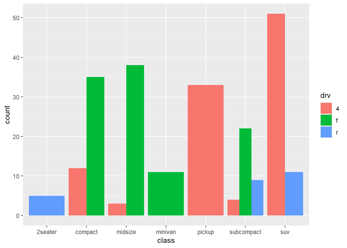
Figure 4.2: Side-by-side bar chart
Notice that all Minivans are front-wheel drive. By default, zero count bars are dropped and the remaining bars are made wider. This may not be the behavior you want. You can modify this using the position = position_dodge(preserve = "single")" option.
library(ggplot2) # grouped bar plot preserving zero count bars ggplot(mpg, aes(x = class, fill = drv)) + geom_bar(position = position_dodge(preserve = "single")) 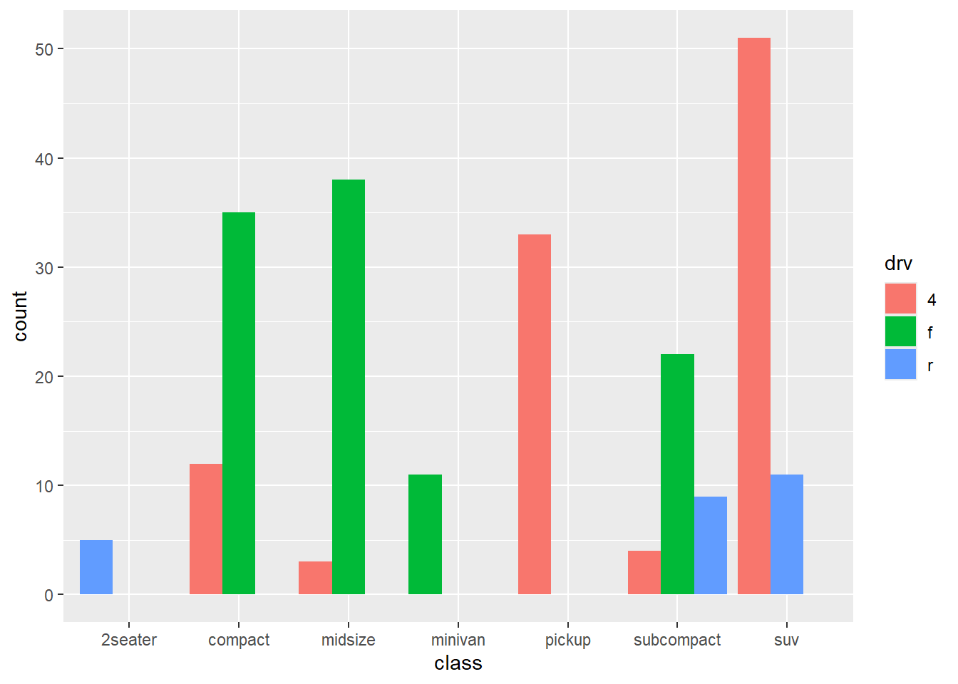
Figure 4.3: Side-by-side bar chart with zero count bars retained
Note that this option is only available in the latest development version of ggplot2, but should should be generally available shortly.
Segmented bar chart
A segmented bar plot is a stacked bar plot where each bar represents 100 percent. You can create a segmented bar chart using the position = "filled" option.
library(ggplot2) # bar plot, with each bar representing 100% ggplot(mpg, aes(x = class, fill = drv)) + geom_bar(position = "fill") + labs(y = "Proportion") 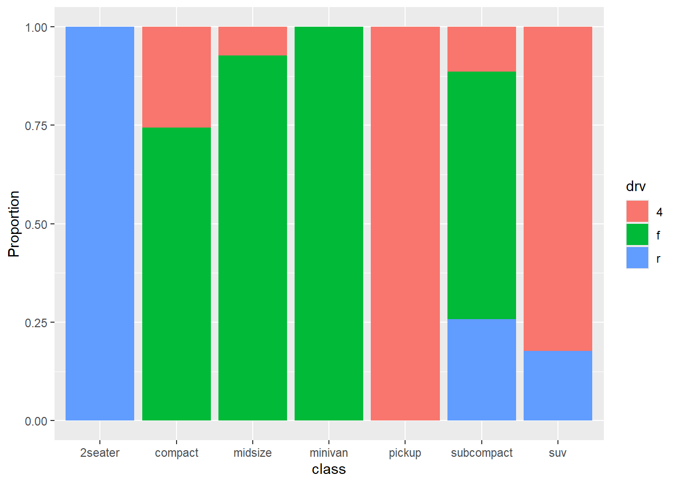
Figure 4.4: Segmented bar chart
This type of plot is particularly useful if the goal is to compare the percentage of a category in one variable across each level of another variable. For example, the proportion of front-wheel drive cars go up as you move from compact, to midsize, to minivan.
Improving the color and labeling
You can use additional options to improve color and labeling. In the graph below
-
factormodifies the order of the categories for the class variable and both the order and the labels for the drive variable
-
scale_y_continuousmodifies the y-axis tick mark labels
-
labsprovides a title and changed the labels for the x and y axes and the legend -
scale_fill_brewerchanges the fill color scheme
-
theme_minimalremoves the grey background and changed the grid color
library(ggplot2) # bar plot, with each bar representing 100%, # reordered bars, and better labels and colors library(scales) ggplot(mpg, aes(x = factor(class, levels = c("2seater", "subcompact", "compact", "midsize", "minivan", "suv", "pickup")), fill = factor(drv, levels = c("f", "r", "4"), labels = c("front-wheel", "rear-wheel", "4-wheel")))) + geom_bar(position = "fill") + scale_y_continuous(breaks = seq(0, 1, .2), label = percent) + scale_fill_brewer(palette = "Set2") + labs(y = "Percent", fill = "Drive Train", x = "Class", title = "Automobile Drive by Class") + theme_minimal() 
Figure 4.5: Segmented bar chart with improved labeling and color
In the graph above, the factor function was used to reorder and/or rename the levels of a categorical variable. You could also apply this to the original dataset, making these changes permanent. It would then apply to all future graphs using that dataset. For example:
# change the order the levels for the categorical variable "class" mpg$class = factor(mpg$class, levels = c("2seater", "subcompact", "compact", "midsize", "minivan", "suv", "pickup") I placed the factor function within the ggplot function to demonstrate that, if desired, you can change the order of the categories and labels for the categories for a single graph.
The other functions are discussed more fully in the section on Customizing graphs.
Next, let's add percent labels to each segment. First, we'll create a summary dataset that has the necessary labels.
# create a summary dataset library(dplyr) plotdata <- mpg %>% group_by(class, drv) %>% summarize(n = n()) %>% mutate(pct = n/ sum(n), lbl = scales:: percent(pct)) plotdata ## # A tibble: 12 x 5 ## # Groups: class [7] ## class drv n pct lbl ## <chr> <chr> <int> <dbl> <chr> ## 1 2seater r 5 1.00 100% ## 2 compact 4 12 0.255 25.5% ## 3 compact f 35 0.745 74.5% ## 4 midsize 4 3 0.0732 7.3% ## 5 midsize f 38 0.927 92.7% ## 6 minivan f 11 1.00 100% ## 7 pickup 4 33 1.00 100% ## 8 subcompact 4 4 0.114 11.4% ## 9 subcompact f 22 0.629 62.9% ## 10 subcompact r 9 0.257 25.7% ## 11 suv 4 51 0.823 82.3% ## 12 suv r 11 0.177 17.7% Next, we'll use this dataset and the geom_text function to add labels to each bar segment.
# create segmented bar chart # adding labels to each segment ggplot(plotdata, aes(x = factor(class, levels = c("2seater", "subcompact", "compact", "midsize", "minivan", "suv", "pickup")), y = pct, fill = factor(drv, levels = c("f", "r", "4"), labels = c("front-wheel", "rear-wheel", "4-wheel")))) + geom_bar(stat = "identity", position = "fill") + scale_y_continuous(breaks = seq(0, 1, .2), label = percent) + geom_text(aes(label = lbl), size = 3, position = position_stack(vjust = 0.5)) + scale_fill_brewer(palette = "Set2") + labs(y = "Percent", fill = "Drive Train", x = "Class", title = "Automobile Drive by Class") + theme_minimal() 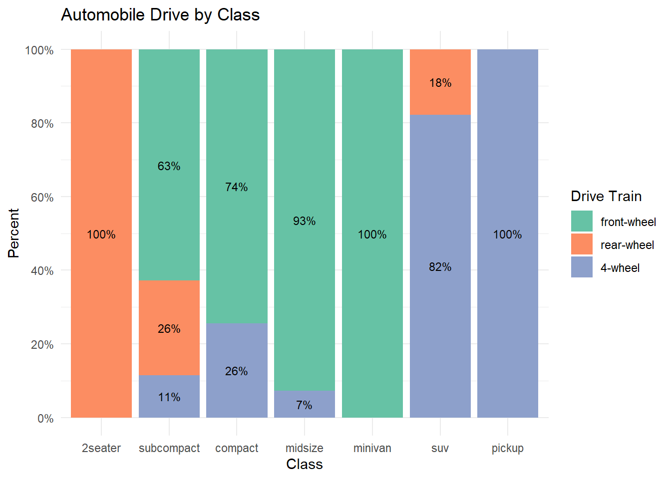
Figure 4.6: Segmented bar chart with value labeling
Now we have a graph that is easy to read and interpret.
Other plots
Mosaic plots provide an alternative to stacked bar charts for displaying the relationship between categorical variables. They can also provide more sophisticated statistical information.
Quantitative vs. Quantitative
The relationship between two quantitative variables is typically displayed using scatterplots and line graphs.
Scatterplot
The simplest display of two quantitative variables is a scatterplot, with each variable represented on an axis. For example, using the Salaries dataset, we can plot experience (yrs.since.phd) vs. academic salary (salary) for college professors.
library(ggplot2) data(Salaries, package= "carData") # simple scatterplot ggplot(Salaries, aes(x = yrs.since.phd, y = salary)) + geom_point() 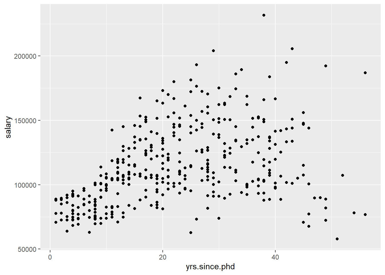
Figure 4.7: Simple scatterplot
geom_point options can be used to change the
-
color- point color -
size- point size -
shape- point shape -
alpha- point transparency. Transparency ranges from 0 (transparent) to 1 (opaque), and is a useful parameter when points overlap.
The functions scale_x_continuous and scale_y_continuous control the scaling on x and y axes respectively.
See Customizing graphs for details.
We can use these options and functions to create a more attractive scatterplot.
# enhanced scatter plot ggplot(Salaries, aes(x = yrs.since.phd, y = salary)) + geom_point(color= "cornflowerblue", size = 2, alpha=.8) + scale_y_continuous(label = scales::dollar, limits = c(50000, 250000)) + scale_x_continuous(breaks = seq(0, 60, 10), limits= c(0, 60)) + labs(x = "Years Since PhD", y = "", title = "Experience vs. Salary", subtitle = "9-month salary for 2008-2009") 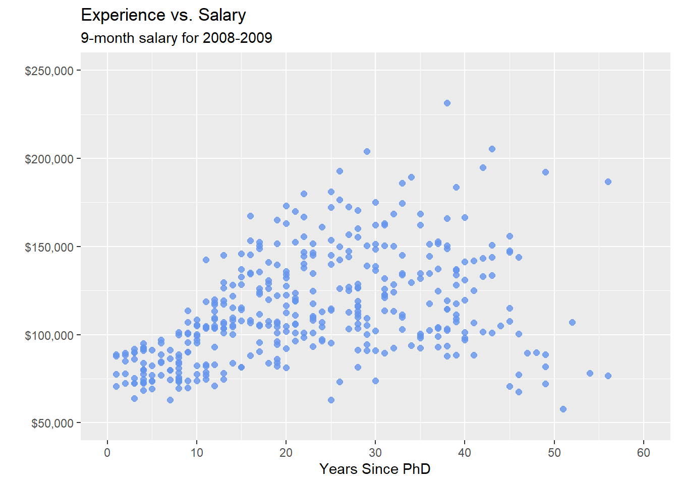
Figure 4.8: Scatterplot with color, transparency, and axis scaling
Adding best fit lines
It is often useful to summarize the relationship displayed in the scatterplot, using a best fit line. Many types of lines are supported, including linear, polynomial, and nonparametric (loess). By default, 95% confidence limits for these lines are displayed.
# scatterplot with linear fit line ggplot(Salaries, aes(x = yrs.since.phd, y = salary)) + geom_point(color= "steelblue") + geom_smooth(method = "lm") 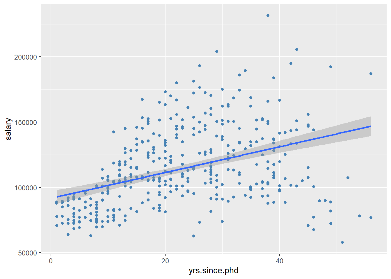
Figure 4.9: Scatterplot with linear fit line
Clearly, salary increases with experience. However, there seems to be a dip at the right end - professors with significant experience, earning lower salaries. A straight line does not capture this non-linear effect. A line with a bend will fit better here.
A polynomial regression line provides a fit line of the form \[\hat{y} = \beta_{0} +\beta_{1}x + \beta{2}x^{2} + \beta{3}x^{3} + \beta{4}x^{4} + \dots\]
Typically either a quadratic (one bend), or cubic (two bends) line is used. It is rarely necessary to use a higher order( >3 ) polynomials. Applying a quadratic fit to the salary dataset produces the following result.
# scatterplot with quadratic line of best fit ggplot(Salaries, aes(x = yrs.since.phd, y = salary)) + geom_point(color= "steelblue") + geom_smooth(method = "lm", formula = y ~ poly(x, 2), color = "indianred3") 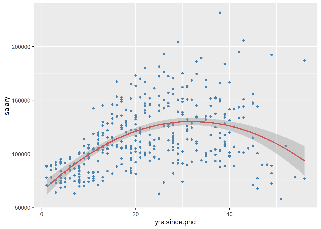
Figure 4.10: Scatterplot with quadratic fit line
Finally, a smoothed nonparametric fit line can often provide a good picture of the relationship. The default in ggplot2 is a loess line which stands for for locally weighted scatterplot smoothing.
# scatterplot with loess smoothed line ggplot(Salaries, aes(x = yrs.since.phd, y = salary)) + geom_point(color= "steelblue") + geom_smooth(color = "tomato") 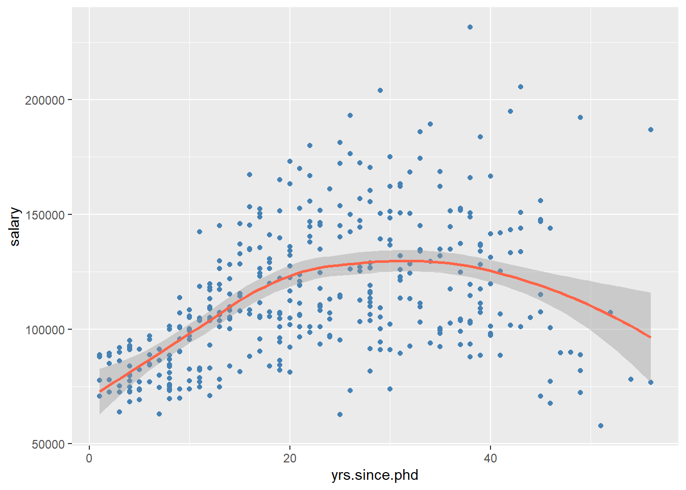
Figure 4.11: Scatterplot with nonparametric fit line
You can suppress the confidence bands by including the option se = FALSE.
Here is a complete (and more attractive) plot.
# scatterplot with loess smoothed line # and better labeling and color ggplot(Salaries, aes(x = yrs.since.phd, y = salary)) + geom_point(color= "cornflowerblue", size = 2, alpha = .6) + geom_smooth(size = 1.5, color = "darkgrey") + scale_y_continuous(label = scales::dollar, limits = c(50000, 250000)) + scale_x_continuous(breaks = seq(0, 60, 10), limits = c(0, 60)) + labs(x = "Years Since PhD", y = "", title = "Experience vs. Salary", subtitle = "9-month salary for 2008-2009") + theme_minimal() 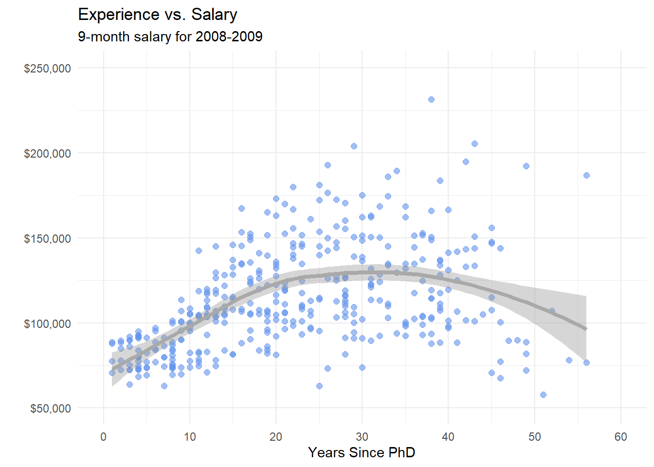
Figure 4.12: Scatterplot with nonparametric fit line
Line plot
When one of the two variables represents time, a line plot can be an effective method of displaying relationship. For example, the code below displays the relationship between time (year) and life expectancy (lifeExp) in the United States between 1952 and 2007. The data comes from the gapminder dataset.
data(gapminder, package= "gapminder") # Select US cases library(dplyr) plotdata <- filter(gapminder, country == "United States") # simple line plot ggplot(plotdata, aes(x = year, y = lifeExp)) + geom_line() 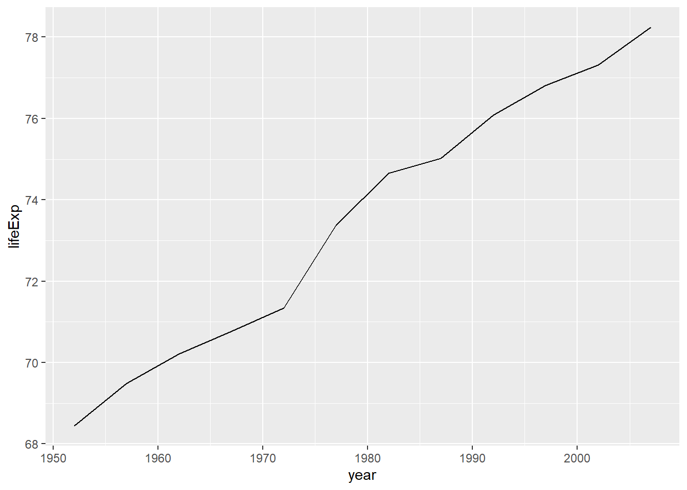
Figure 4.13: Simple line plot
It is hard to read individual values in the graph above. In the next plot, we'll add points as well.
# line plot with points # and improved labeling ggplot(plotdata, aes(x = year, y = lifeExp)) + geom_line(size = 1.5, color = "lightgrey") + geom_point(size = 3, color = "steelblue") + labs(y = "Life Expectancy (years)", x = "Year", title = "Life expectancy changes over time", subtitle = "United States (1952-2007)", caption = "Source: http://www.gapminder.org/data/") 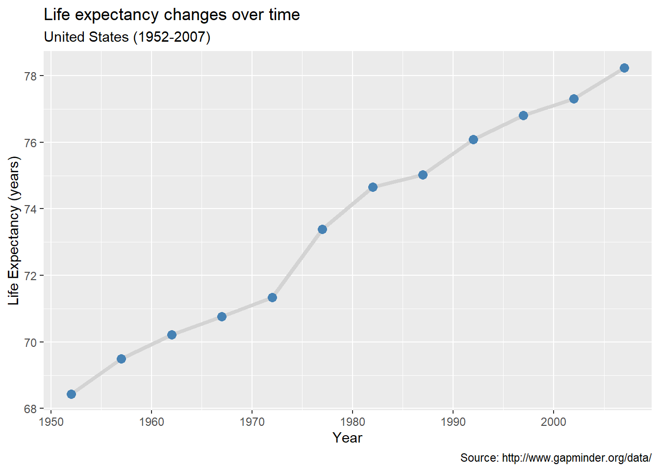
Figure 4.14: Line plot with points and labels
Time dependent data is covered in more detail under Time series. Customizing line graphs is covered in the Customizing graphs section.
Categorical vs. Quantitative
When plotting the relationship between a categorical variable and a quantitative variable, a large number of graph types are available. These include bar charts using summary statistics, grouped kernel density plots, side-by-side box plots, side-by-side violin plots, mean/sem plots, ridgeline plots, and Cleveland plots.
Bar chart (on summary statistics)
In previous sections, bar charts were used to display the number of cases by category for a single variable or for two variables. You can also use bar charts to display other summary statistics (e.g., means or medians) on a quantitative variable for each level of a categorical variable.
For example, the following graph displays the mean salary for a sample of university professors by their academic rank.
data(Salaries, package= "carData") # calculate mean salary for each rank library(dplyr) plotdata <- Salaries %>% group_by(rank) %>% summarize(mean_salary = mean(salary)) # plot mean salaries ggplot(plotdata, aes(x = rank, y = mean_salary)) + geom_bar(stat = "identity") 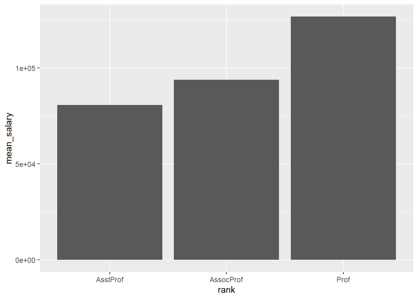
Figure 4.15: Bar chart displaying means
We can make it more attractive with some options.
# plot mean salaries in a more attractive fashion library(scales) ggplot(plotdata, aes(x = factor(rank, labels = c("Assistant \n Professor", "Associate \n Professor", "Full \n Professor")), y = mean_salary)) + geom_bar(stat = "identity", fill = "cornflowerblue") + geom_text(aes(label = dollar(mean_salary)), vjust = - 0.25) + scale_y_continuous(breaks = seq(0, 130000, 20000), label = dollar) + labs(title = "Mean Salary by Rank", subtitle = "9-month academic salary for 2008-2009", x = "", y = "") 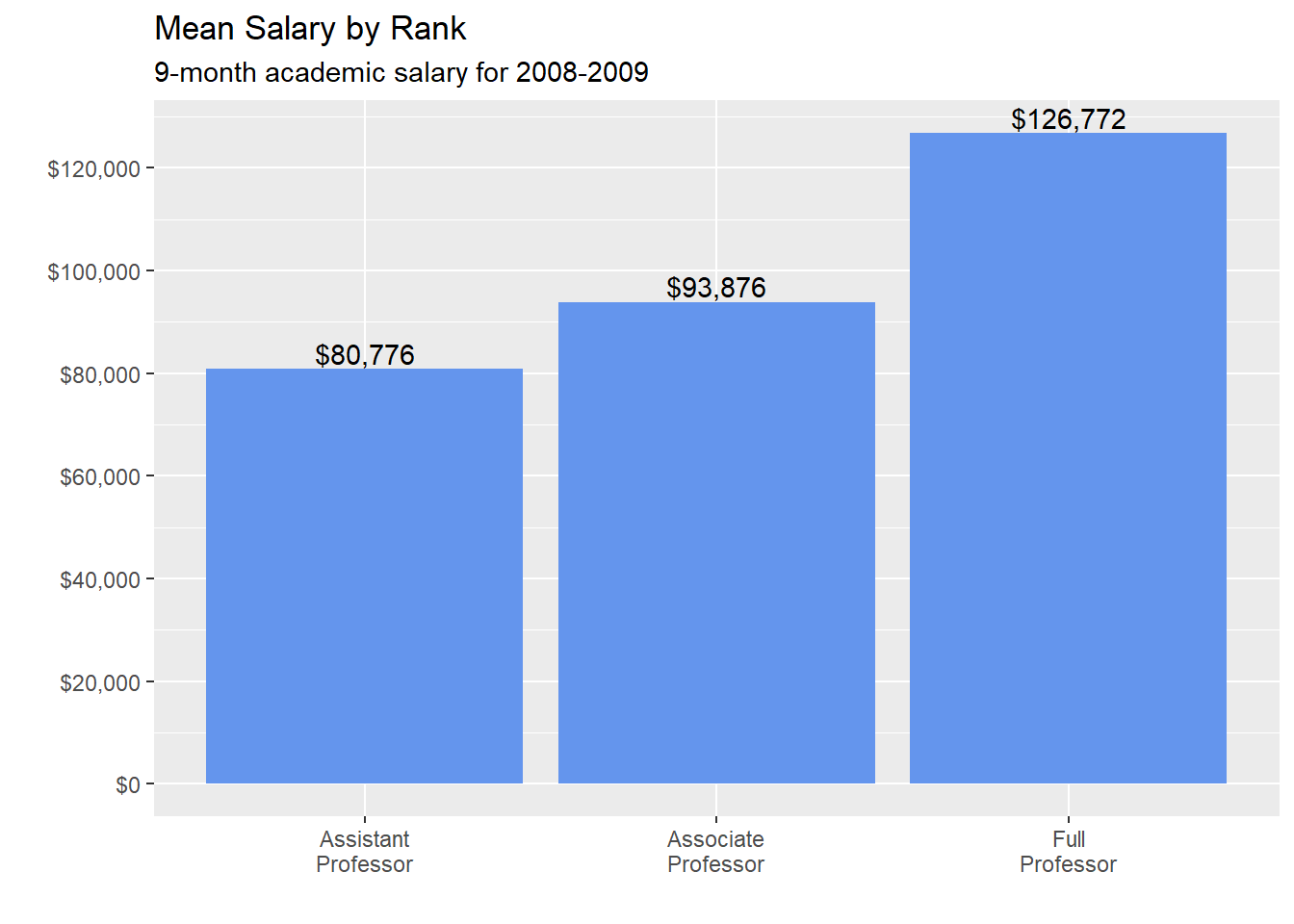
Figure 4.16: Bar chart displaying means
One limitation of such plots is that they do not display the distribution of the data - only the summary statistic for each group. The plots below correct this limitation to some extent.
Grouped kernel density plots
One can compare groups on a numeric variable by superimposing kernel density plots in a single graph.
# plot the distribution of salaries # by rank using kernel density plots ggplot(Salaries, aes(x = salary, fill = rank)) + geom_density(alpha = 0.4) + labs(title = "Salary distribution by rank") 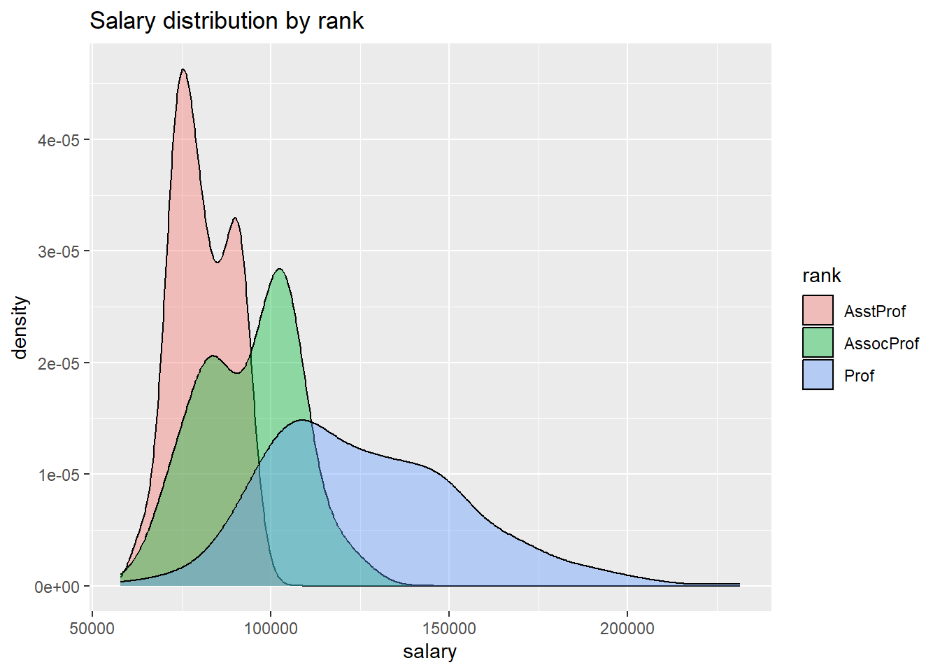
Figure 4.17: Grouped kernel density plots
The alpha option makes the density plots partially transparent, so that we can see what is happening under the overlaps. Alpha values range from 0 (transparent) to 1 (opaque). The graph makes clear that, in general, salary goes up with rank. However, the salary range for full professors is very wide.
Box plots
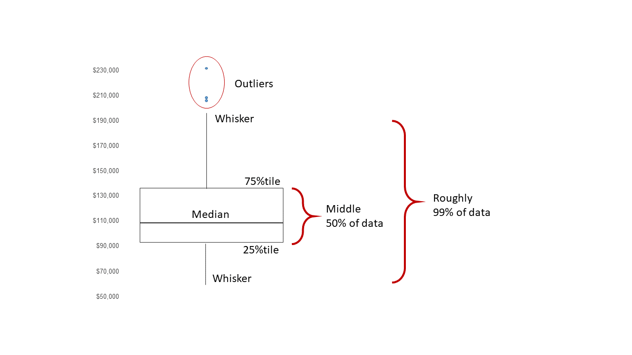
A boxplot displays the 25th percentile, median, and 75th percentile of a distribution. The whiskers (vertical lines) capture roughly 99% of a normal distribution, and observations outside this range are plotted as points representing outliers (see the figure below).
 Side-by-side box plots are very useful for comparing groups (i.e., the levels of a categorical variable) on a numerical variable.
# plot the distribution of salaries by rank using boxplots ggplot(Salaries, aes(x = rank, y = salary)) + geom_boxplot() + labs(title = "Salary distribution by rank") 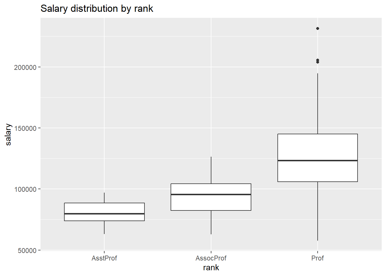
Figure 4.18: Side-by-side boxplots
Notched boxplots provide an approximate method for visualizing whether groups differ. Although not a formal test, if the notches of two boxplots do not overlap, there is strong evidence (95% confidence) that the medians of the two groups differ.
# plot the distribution of salaries by rank using boxplots ggplot(Salaries, aes(x = rank, y = salary)) + geom_boxplot(notch = TRUE, fill = "cornflowerblue", alpha = .7) + labs(title = "Salary distribution by rank") 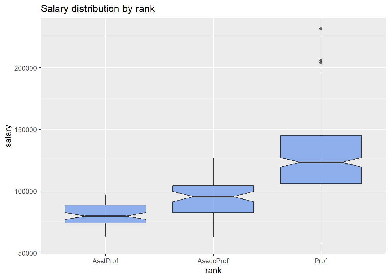
Figure 4.19: Side-by-side notched boxplots
In the example above, all three groups appear to differ.
One of the advantages of boxplots is that their widths are not usually meaningful. This allows you to compare the distribution of many groups in a single graph.
Violin plots
Violin plots are similar to kernel density plots, but are mirrored and rotated 90o.
# plot the distribution of salaries # by rank using violin plots ggplot(Salaries, aes(x = rank, y = salary)) + geom_violin() + labs(title = "Salary distribution by rank") 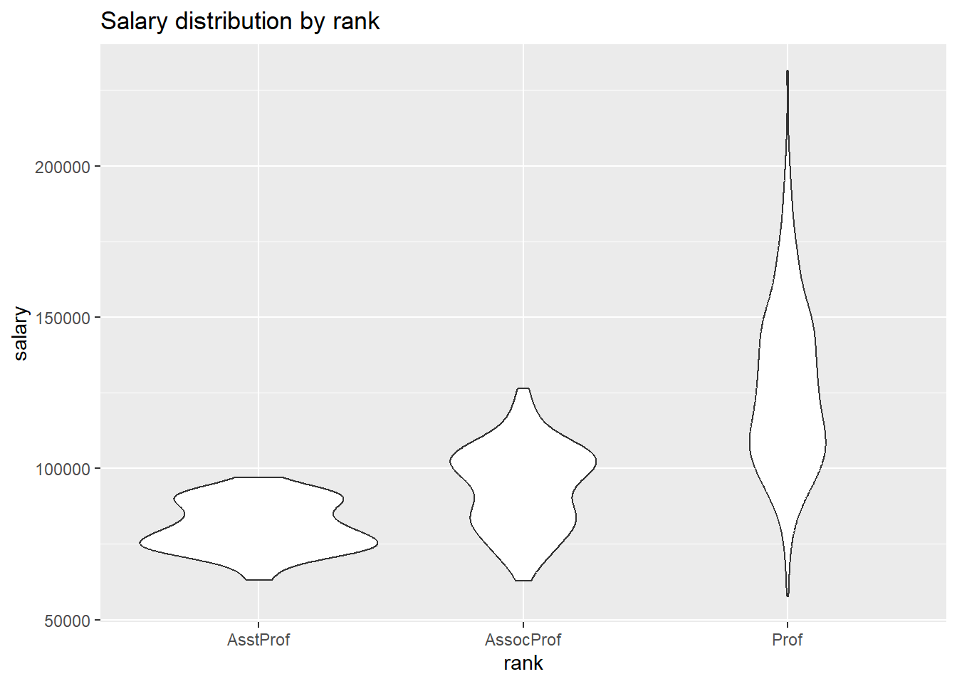
Figure 4.20: Side-by-side violin plots
A useful variation is to superimpose boxplots on violin plots.
# plot the distribution using violin and boxplots ggplot(Salaries, aes(x = rank, y = salary)) + geom_violin(fill = "cornflowerblue") + geom_boxplot(width = .2, fill = "orange", outlier.color = "orange", outlier.size = 2) + labs(title = "Salary distribution by rank") 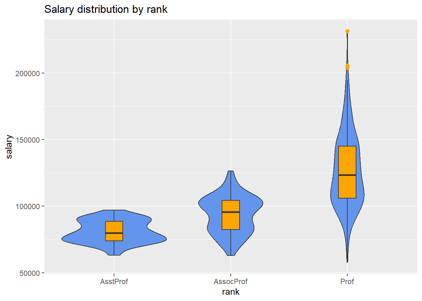
Figure 4.21: Side-by-side violin/box plots
Ridgeline plots
A ridgeline plot (also called a joyplot) displays the distribution of a quantitative variable for several groups. They're similar to kernel density plots with vertical faceting, but take up less room. Ridgeline plots are created with the ggridges package.
Using the Fuel economy dataset, let's plot the distribution of city driving miles per gallon by car class.
# create ridgeline graph library(ggplot2) library(ggridges) ggplot(mpg, aes(x = cty, y = class, fill = class)) + geom_density_ridges() + theme_ridges() + labs("Highway mileage by auto class") + theme(legend.position = "none") 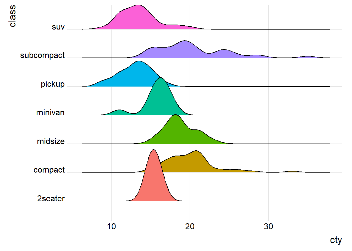
Figure 4.22: Ridgeline graph with color fill
I've suppressed the legend here because it's redundant (the distributions are already labeled on the y-axis). Unsurprisingly, pickup trucks have the poorest mileage, while subcompacts and compact cars tend to achieve ratings. However, there is a very wide range of gas mileage scores for these smaller cars.
Note the the possible overlap of distributions is the trade-off for a more compact graph. You can add transparency if the the overlap is severe using geom_density_ridges(alpha = n), where n ranges from 0 (transparent) to 1 (opaque). See the package vingnette for more details.
Mean/SEM plots
A popular method for comparing groups on a numeric variable is the mean plot with error bars. Error bars can represent standard deviations, standard error of the mean, or confidence intervals. In this section, we'll plot means and standard errors.
# calculate means, standard deviations, # standard errors, and 95% confidence # intervals by rank library(dplyr) plotdata <- Salaries %>% group_by(rank) %>% summarize(n = n(), mean = mean(salary), sd = sd(salary), se = sd / sqrt(n), ci = qt(0.975, df = n - 1) * sd / sqrt(n)) The resulting dataset is given below.
| rank | n | mean | sd | se | ci |
|---|---|---|---|---|---|
| AsstProf | 67 | 80775.99 | 8174.113 | 998.6268 | 1993.823 |
| AssocProf | 64 | 93876.44 | 13831.700 | 1728.9625 | 3455.056 |
| Prof | 266 | 126772.11 | 27718.675 | 1699.5410 | 3346.322 |
# plot the means and standard errors ggplot(plotdata, aes(x = rank, y = mean, group = 1)) + geom_point(size = 3) + geom_line() + geom_errorbar(aes(ymin = mean - se, ymax = mean + se), width = .1) 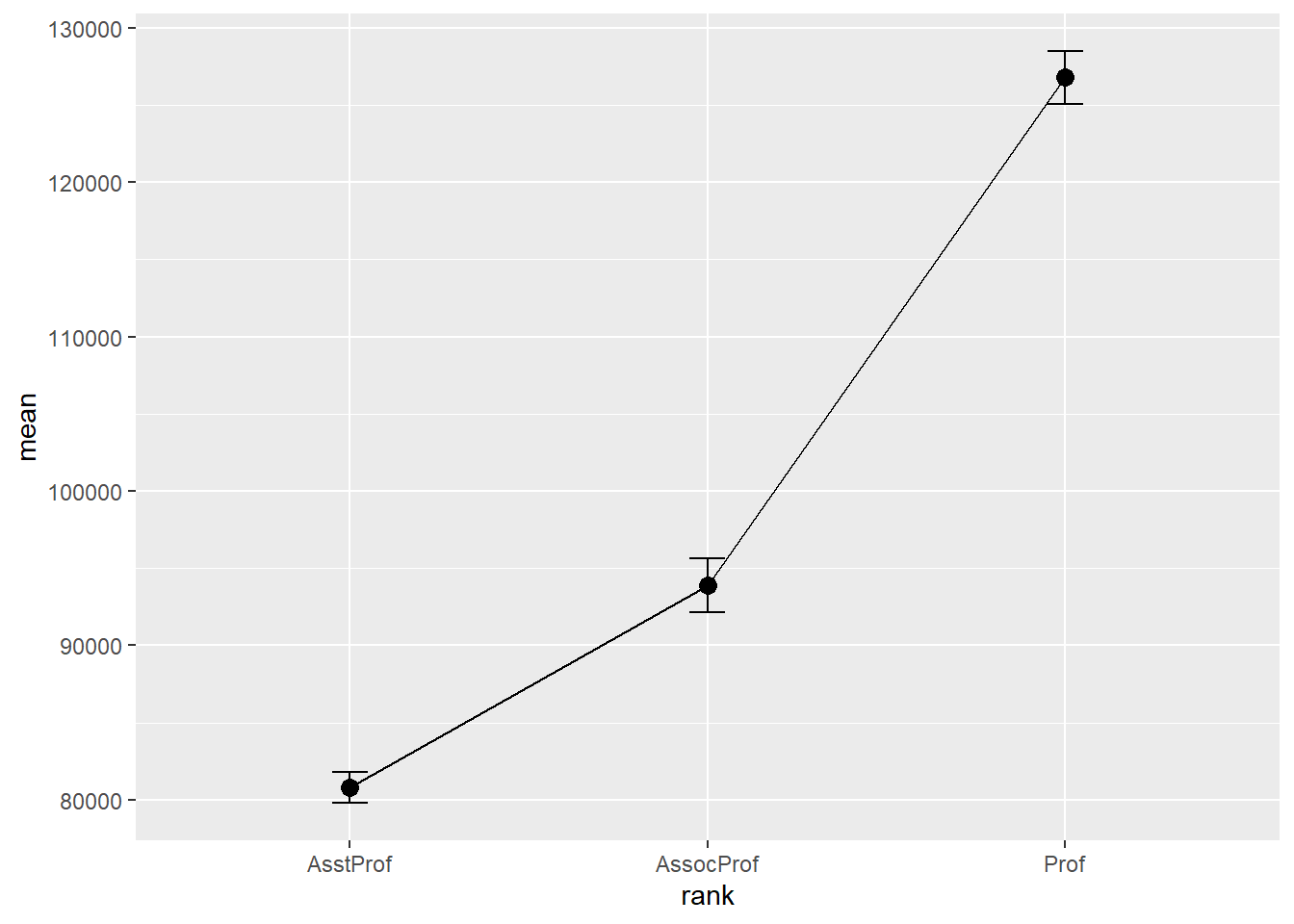
Figure 4.23: Mean plots with standard error bars
Although we plotted error bars representing the standard error, we could have plotted standard deviations or 95% confidence intervals. Simply replace se with sd or error in the aes option.
We can use the same technique to compare salary across rank and sex. (Technically, this is not bivariate since we're plotting rank, sex, and salary, but it seems to fit here)
# calculate means and standard errors by rank and sex plotdata <- Salaries %>% group_by(rank, sex) %>% summarize(n = n(), mean = mean(salary), sd = sd(salary), se = sd/ sqrt(n)) # plot the means and standard errors by sex ggplot(plotdata, aes(x = rank, y = mean, group=sex, color=sex)) + geom_point(size = 3) + geom_line(size = 1) + geom_errorbar(aes(ymin =mean - se, ymax = mean+se), width = .1) 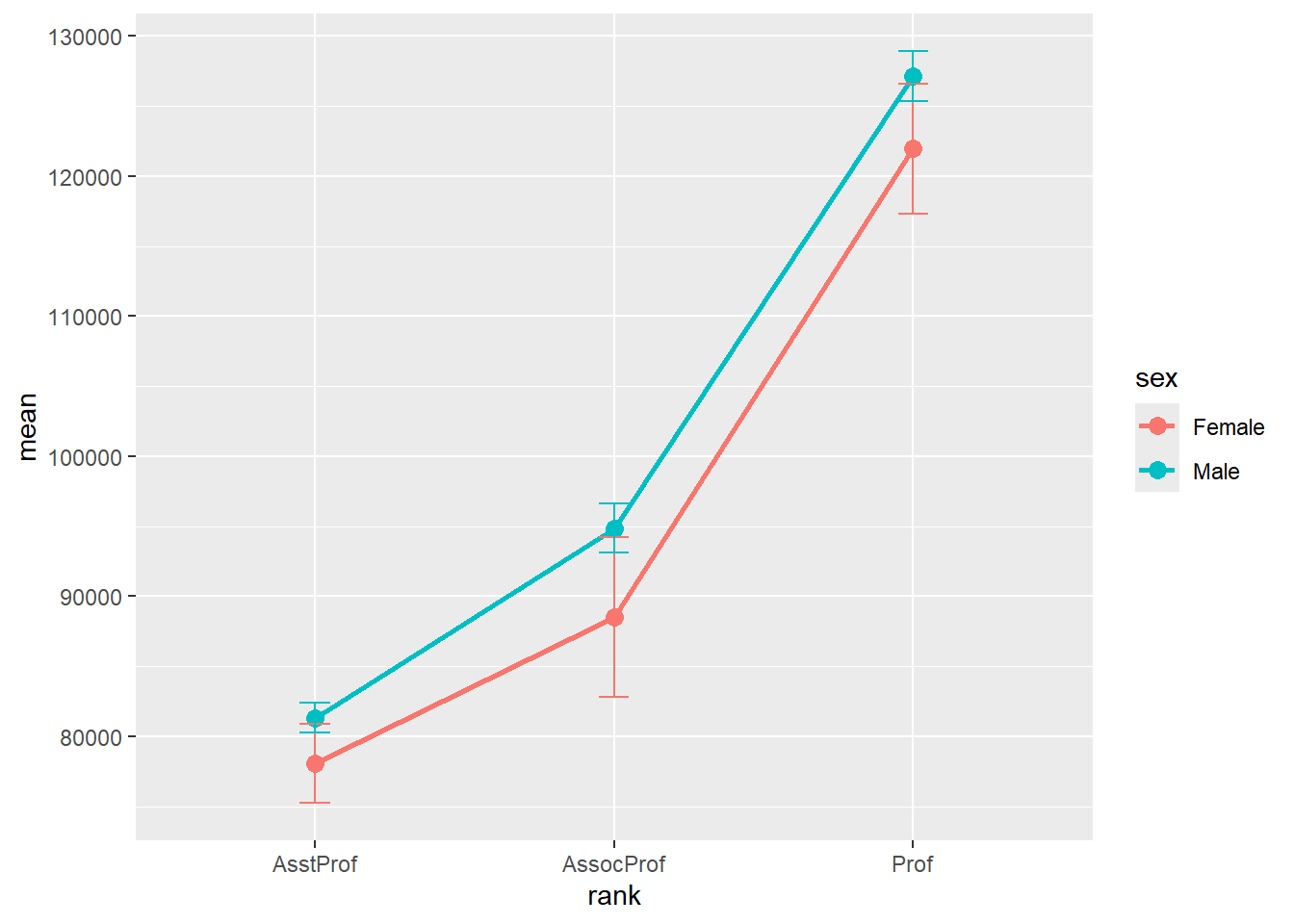
Figure 4.24: Mean plots with standard error bars by sex
Unfortunately, the error bars overlap. We can dodge the horizontal positions a bit to overcome this.
# plot the means and standard errors by sex (dodged) pd <- position_dodge(0.2) ggplot(plotdata, aes(x = rank, y = mean, group=sex, color=sex)) + geom_point(position = pd, size = 3) + geom_line(position = pd, size = 1) + geom_errorbar(aes(ymin = mean - se, ymax = mean + se), width = .1, position= pd) 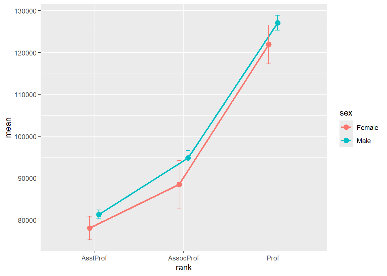
Figure 4.25: Mean plots with standard error bars (dodged)
Finally, lets add some options to make the graph more attractive.
# improved means/standard error plot pd <- position_dodge(0.2) ggplot(plotdata, aes(x = factor(rank, labels = c("Assistant \n Professor", "Associate \n Professor", "Full \n Professor")), y = mean, group=sex, color=sex)) + geom_point(position=pd, size = 3) + geom_line(position = pd, size = 1) + geom_errorbar(aes(ymin = mean - se, ymax = mean + se), width = .1, position = pd, size = 1) + scale_y_continuous(label = scales::dollar) + scale_color_brewer(palette= "Set1") + theme_minimal() + labs(title = "Mean salary by rank and sex", subtitle = "(mean +/- standard error)", x = "", y = "", color = "Gender") 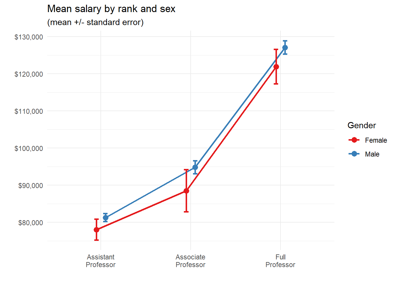
Figure 4.26: Mean/se plot with better labels and colors
Strip plots
The relationship between a grouping variable and a numeric variable can be displayed with a scatter plot. For example
# plot the distribution of salaries # by rank using strip plots ggplot(Salaries, aes(y = rank, x = salary)) + geom_point() + labs(title = "Salary distribution by rank") 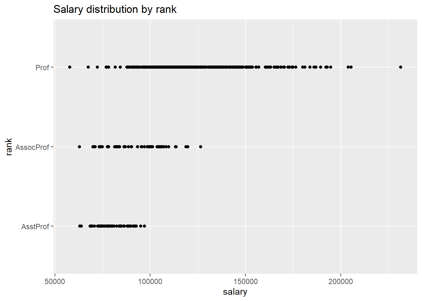
Figure 4.27: Categorical by quantiative scatterplot
These one-dimensional scatterplots are called strip plots. Unfortunately, overprinting of points makes interpretation difficult. The relationship is easier to see if the the points are jittered. Basically a small random number is added to each y-coordinate.
# plot the distribution of salaries # by rank using jittering ggplot(Salaries, aes(y = rank, x = salary)) + geom_jitter() + labs(title = "Salary distribution by rank") 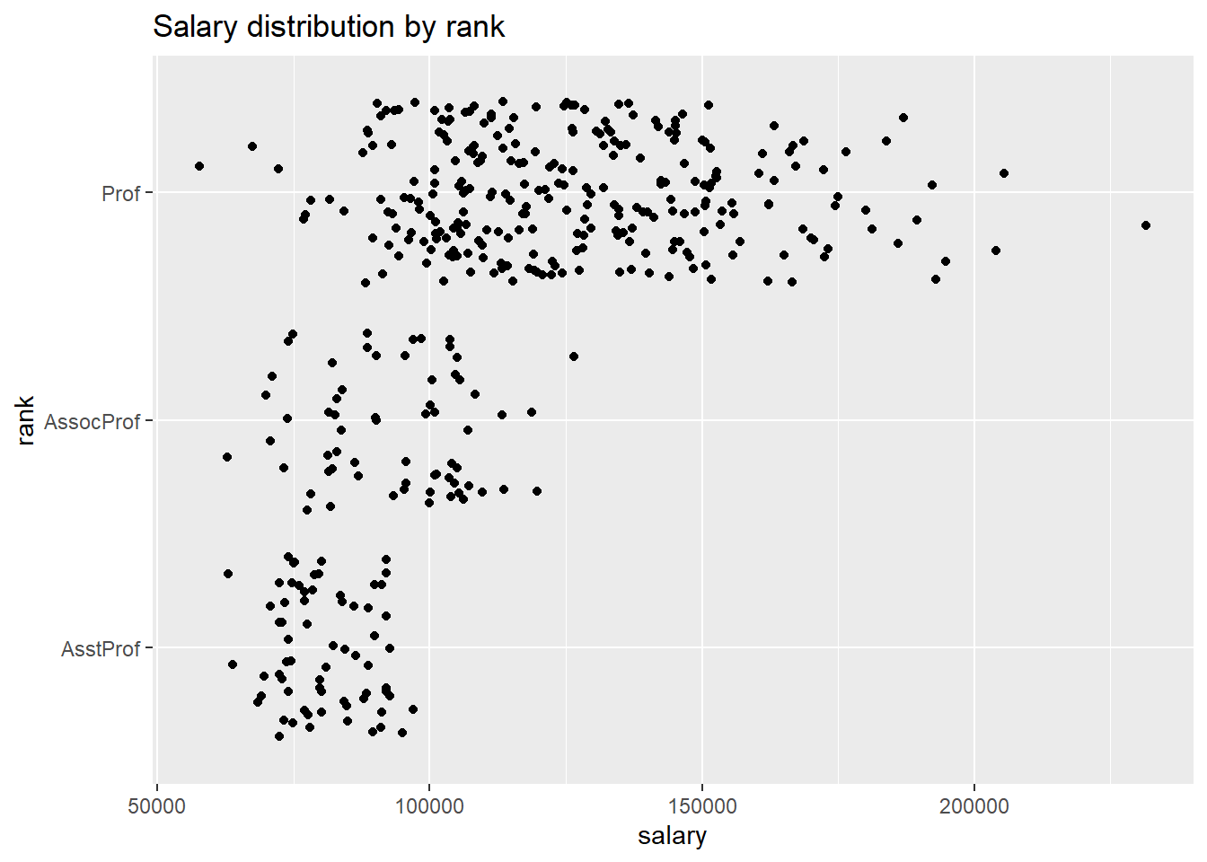
Figure 4.28: Jittered plot
It is easier to compare groups if we use color.
# plot the distribution of salaries # by rank using jittering library(scales) ggplot(Salaries, aes(y = factor(rank, labels = c("Assistant \n Professor", "Associate \n Professor", "Full \n Professor")), x = salary, color = rank)) + geom_jitter(alpha = 0.7, size = 1.5) + scale_x_continuous(label = dollar) + labs(title = "Academic Salary by Rank", subtitle = "9-month salary for 2008-2009", x = "", y = "") + theme_minimal() + theme(legend.position = "none") 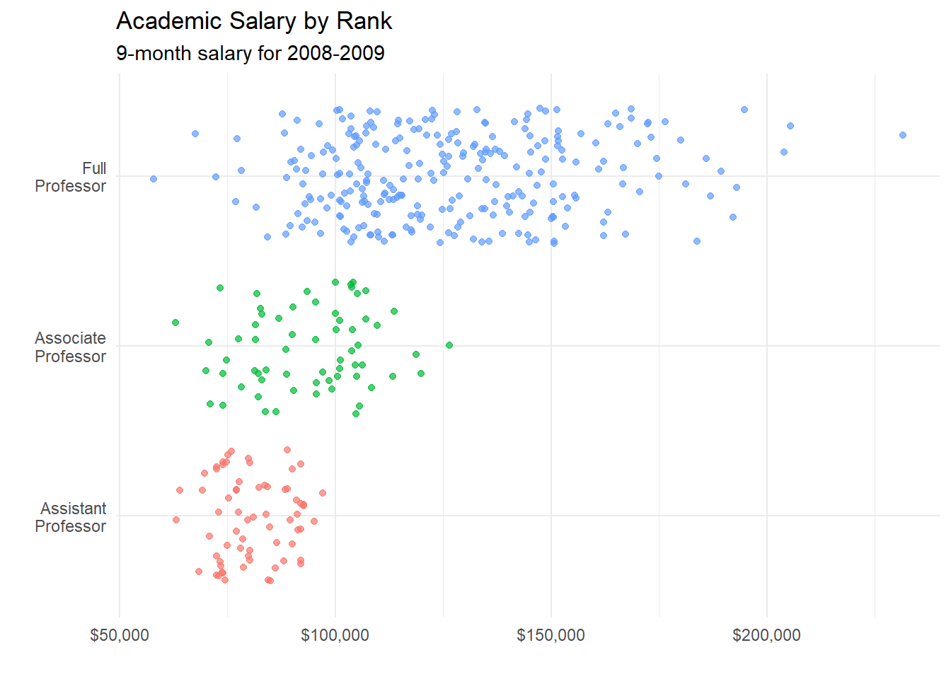
Figure 4.29: Fancy jittered plot
The option legend.position = "none" is used to suppress the legend (which is not needed here). Jittered plots work well when the number of points in not overly large.
Combining jitter and boxplots
It may be easier to visualize distributions if we add boxplots to the jitter plots.
# plot the distribution of salaries # by rank using jittering library(scales) ggplot(Salaries, aes(x = factor(rank, labels = c("Assistant \n Professor", "Associate \n Professor", "Full \n Professor")), y = salary, color = rank)) + geom_boxplot(size= 1, outlier.shape = 1, outlier.color = "black", outlier.size = 3) + geom_jitter(alpha = 0.5, width=.2) + scale_y_continuous(label = dollar) + labs(title = "Academic Salary by Rank", subtitle = "9-month salary for 2008-2009", x = "", y = "") + theme_minimal() + theme(legend.position = "none") + coord_flip() 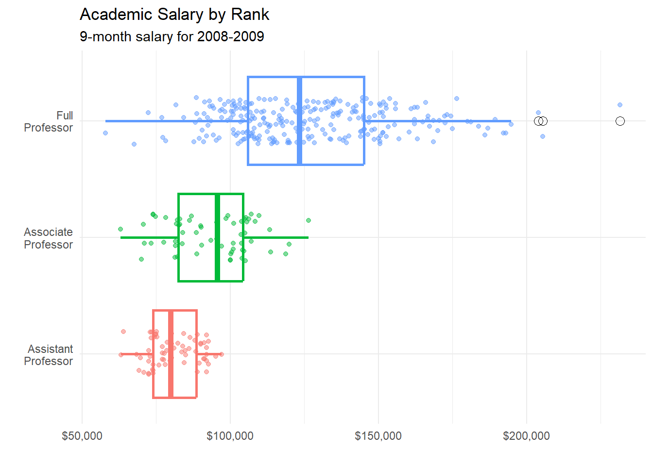
Figure 4.30: Jitter plot with superimposed box plots
Several options were added to create this plot.
For the boxplot
-
size = 1makes the lines thicker
-
outlier.color = "black"makes outliers black -
outlier.shape = 1specifies circles for outliers -
outlier.size = 3increases the size of the outlier symbol
For the jitter
-
alpha = 0.5makes the points more transparent -
width = .2decreases the amount of jitter (.4 is the default)
Finally, the x and y axes are revered using the coord_flip function (i.e., the graph is turned on its side).
Before moving on, it is worth mentioning the geom_boxjitter function provided in the ggpol package. It creates a hybrid boxplot - half boxplot, half scatterplot.
# plot the distribution of salaries # by rank using jittering library(ggpol) library(scales) ggplot(Salaries, aes(x = factor(rank, labels = c("Assistant \n Professor", "Associate \n Professor", "Full \n Professor")), y = salary, fill=rank)) + geom_boxjitter(color= "black", jitter.color = "darkgrey", errorbar.draw = TRUE) + scale_y_continuous(label = dollar) + labs(title = "Academic Salary by Rank", subtitle = "9-month salary for 2008-2009", x = "", y = "") + theme_minimal() + theme(legend.position = "none") 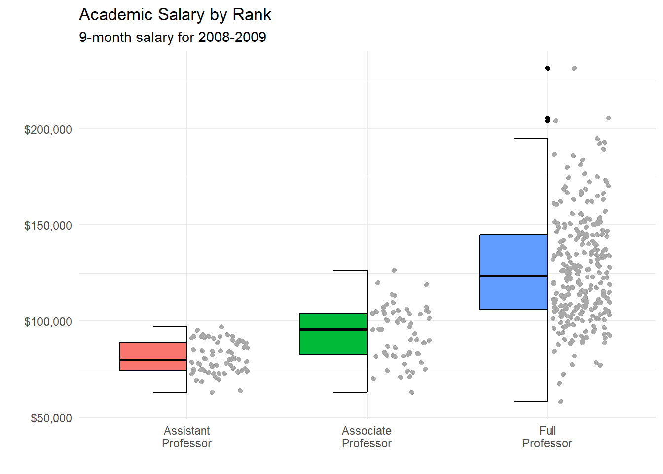
Figure 4.31: Using geom_boxjitter
Beeswarm Plots
Beeswarm plots (also called violin scatter plots) are similar to jittered scatterplots, in that they display the distribution of a quantitative variable by plotting points in way that reduces overlap. In addition, they also help display the density of the data at each point (in a manner that is similar to a violin plot). Continuing the previous example
# plot the distribution of salaries # by rank using beewarm-syle plots library(ggbeeswarm) library(scales) ggplot(Salaries, aes(x = factor(rank, labels = c("Assistant \n Professor", "Associate \n Professor", "Full \n Professor")), y = salary, color = rank)) + geom_quasirandom(alpha = 0.7, size = 1.5) + scale_y_continuous(label = dollar) + labs(title = "Academic Salary by Rank", subtitle = "9-month salary for 2008-2009", x = "", y = "") + theme_minimal() + theme(legend.position = "none") 
Figure 4.32: Beeswarm plot
The plots are create using the geom_quasirandom function. These plots can be easier to read than simple jittered strip plots. To learn more about these plots, see Beeswarm-style plots with ggplot2.
Cleveland Dot Charts
Cleveland plots are useful when you want to compare a numeric statistic for a large number of groups. For example, say that you want to compare the 2007 life expectancy for Asian country using the gapminder dataset.
data(gapminder, package= "gapminder") # subset Asian countries in 2007 library(dplyr) plotdata <- gapminder %>% filter(continent == "Asia" & year == 2007) # basic Cleveland plot of life expectancy by country ggplot(plotdata, aes(x= lifeExp, y = country)) + geom_point() 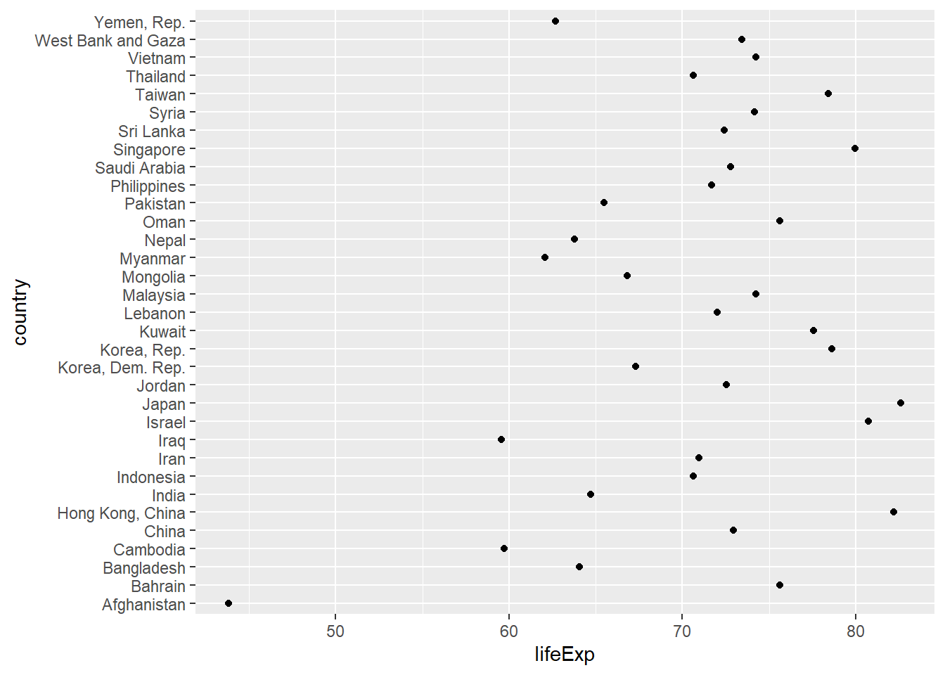
Figure 4.33: Basic Cleveland dot plot
Comparisons are usually easier if the y-axis is sorted.
# Sorted Cleveland plot ggplot(plotdata, aes(x=lifeExp, y= reorder(country, lifeExp))) + geom_point() 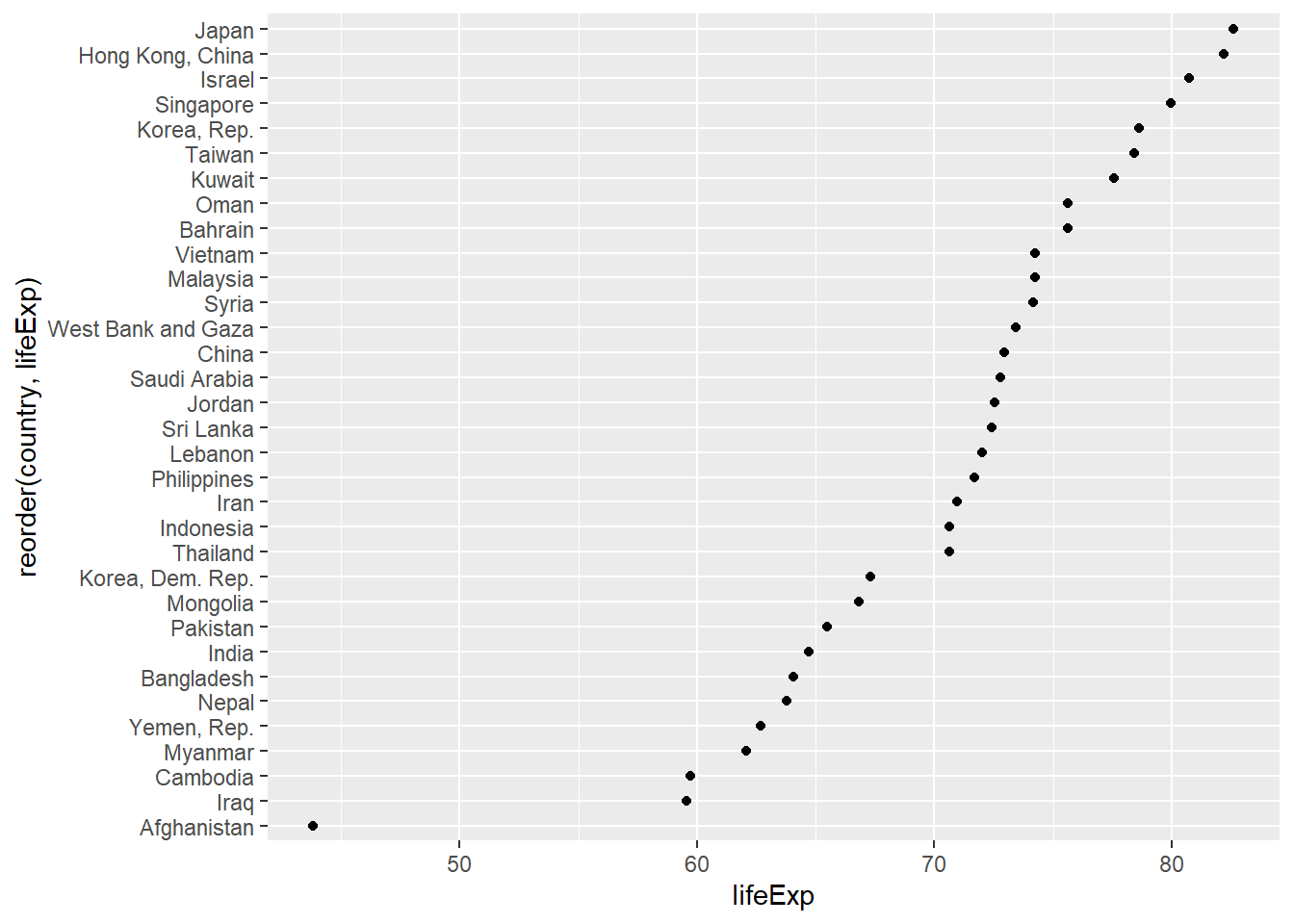
Figure 4.34: Sorted Cleveland dot plot
Finally, we can use options to make the graph more attractive.
# Fancy Cleveland plot ggplot(plotdata, aes(x=lifeExp, y= reorder(country, lifeExp))) + geom_point(color= "blue", size = 2) + geom_segment(aes(x = 40, xend = lifeExp, y = reorder(country, lifeExp), yend = reorder(country, lifeExp)), color = "lightgrey") + labs (x = "Life Expectancy (years)", y = "", title = "Life Expectancy by Country", subtitle = "GapMinder data for Asia - 2007") + theme_minimal() + theme(panel.grid.major = element_blank(), panel.grid.minor = element_blank()) 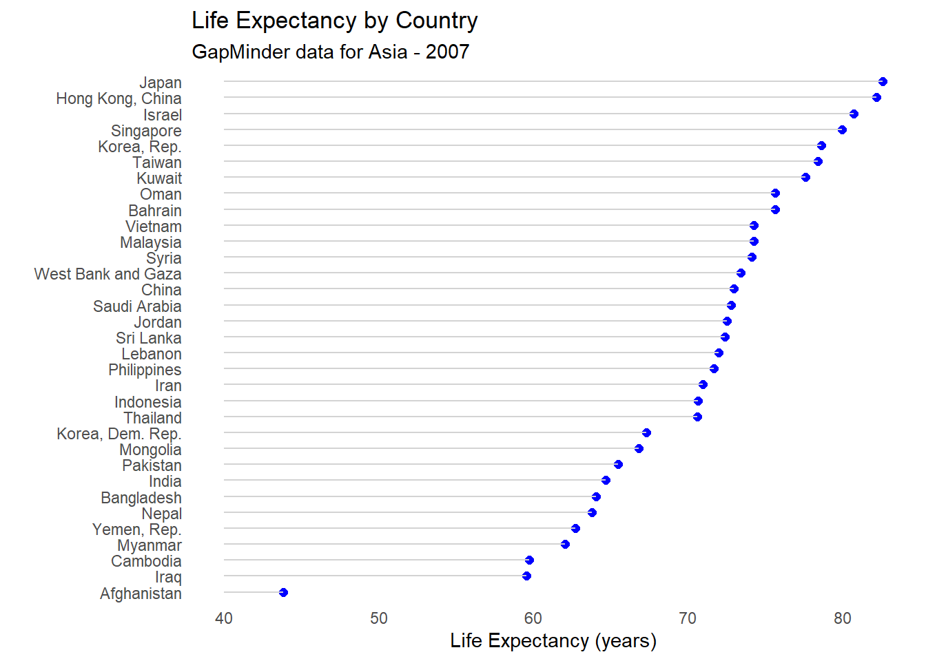
Figure 4.35: Fancy Cleveland plot
Japan clearly has the highest life expectancy, while Afghanistan has the lowest by far. This last plot is also called a lollipop graph (you can see why).
Source: https://rkabacoff.github.io/datavis/Bivariate.html
0 Response to "How to Make Bar Graph of Continuous Data R Count"
Post a Comment